alex   >>> /Users/epolyach/Dropbox/WORK/HTML/; /Users/epolyach/Dropbox/Urtica/Nbody/LossCone/polynomial_df/
edita  >>> /home/epolyach/Dropbox/JOB/HTML/; /home/epolyach/Data/WORK/LC_harm/
kepler >>> /home/Tit2/berczik/Evgeny-harm/; /home/Tit5/epolyach/VW/Harmonic

Loss cone paper

Among tasks of year 1 of our VW trilateral project there is:

Theoretical input

As a first step, we decided to model the simplest Polyanomial DF:

\[ \begin{equation} F = N \delta(E-E_0) \alpha^n\ ,\quad \alpha \equiv L/L_\textrm{circ}\ . \label{eq:DF} \end{equation} \]

The resulting density distribution is:

\[ \begin{equation} \rho \propto r^n (1-r^2)^{(n+1)/2}\ . \end{equation} \]

This stellar cluster is embedded to the dominating harmonic potential, so the total potential is

\[ \begin{equation} \Phi_0(r) = \frac{\Omega_0^2 r^2}{2} + \Phi_G(r)\ . \label{eq:Pot} \end{equation} \]

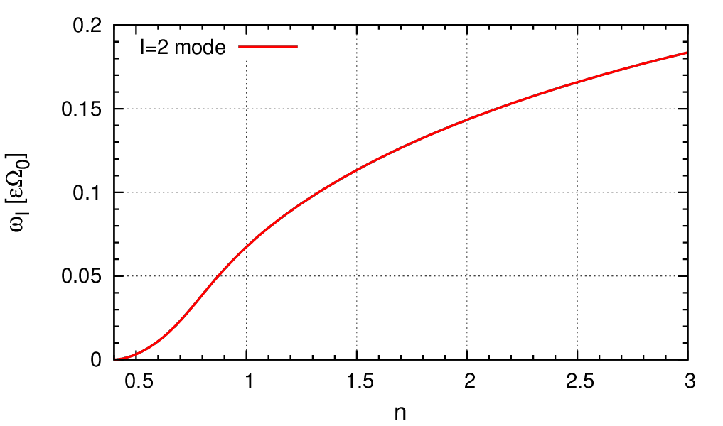
Theoretical prediction of the growth rate:

Here the issue is two timescales. The first one is the dynamical timescale:

\[ t_\textrm{dyn} \sim \Omega_0^{-1}\ . \]

The other one is the precession or secular timescale:

\[ t_\textrm{sec} \sim (\epsilon \Omega_0)^{-1}\ , \quad \epsilon \equiv \frac{G M_G}{R^3 \Omega_0^2} \]

In the upper figure, there are slow units measured in units \(\epsilon \Omega_0\).

Two body relaxation time (BT, p. 587):

\[ \frac{t_\textrm{relax}}{t_\textrm{dyn}} = \frac{0.34 \sigma^3}{G^2 m\rho \ln \Lambda } \frac1{t_\textrm{dyn}}\ , \]

where \(\sigma^2\) is is the mean-square velocity in any one direction, is estimated here as (\(\sigma \sim \Omega_0 R\), \(m=M_G/N\), \(\rho \sim 3 M_G/(4\pi R^3)\) ):

\[ \frac{t_\textrm{relax}}{t_\textrm{dyn}} \sim \frac{N}{\ln \Lambda} \frac{\Omega_0^4}{\Omega^4_\textrm{sg}}\ , \quad \Omega^2_\textrm{sg} \equiv \frac{G M_G}{R^3} \]

The energies of the stars diffuse on this timescale.

Because the harmonic ellipse traced out by a star is approximately fixed on a timescale \(t_\textrm{sec}\), the average torque between two stars is approximately constant over this timescale. This slow variation in the mutual torques between stars gives rise to enhanced or resonant relaxation of the angular momenta (Rauch & Tremaine 1996); the corresponding timescale is (Tremaine 2005):

\[ \frac{t_\textrm{res}}{t_\textrm{dyn}} \sim N \frac{\Omega_0^2}{\Omega^2_\textrm{sg}} \ . \]

Initial Particle Distribution (IPD)

The DF is in equilibrium by construction. \(G=M_G=1\); \(\Omega_0\) is a characteristic of the halo. The routine I use for creating the DF calculates a library of orbits (let ‘NL’ be the number of orbits in the library) in the allowed range over \(L\), then after playing the angular momentum, it interpolates between the orbits to produce \(r\) out of the radial angle \(w\). Once we have \(r\), we easily have \(v_r\), \(v_\perp\), and then all we need.

Note that I do not account for the softening, i.e. introducing softening we violate equilibrium. But Peter checked that softening \(\epsilon=0.001\) is almost the same as our default softening 0.005, and 0.025 differs only slightly if we compare amplitudes of the quadrupole harmonic. So for the moment, we think that softening is not an issue. We adopt \(\epsilon=0.005\) for the future runs.

N-body modelling

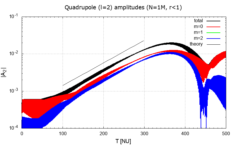
For \(n=2\), theory predicts the growth rate of the quadrupole perturbations \(\omega_\textrm{I} \approx 0.14\). We made several N-body runs of the model with this value of \(n\) using \(\Omega_0=10\) in units \(G=M_G=R=1\), where \(M_G\) is the cluster mass, \(R\) is the outer radius. In these units, the dynamical time is 0.1, the secular time is 10, the two-body relaxation time is of the order of \(10^{7}\), as well as the resonance relaxation time for \(N=1\)M run (see figures for 200k run here).

It is seen that the run with 1M particles reproduces the growth rate quite well. However, the amplitude falls off the straight line early. The instability disappears on the level \(\sim 10^{-2}\), when the distortion is not seen by eye. (The green line is well below \(10^{-4}\).)

Figure 1.

Energy diffusion

Figure 2. This is how the energy distribution spreads with time. Here is one for 1M run, the selfgravitating potential is set to zero at infinity, so \(E_0 = 49\):

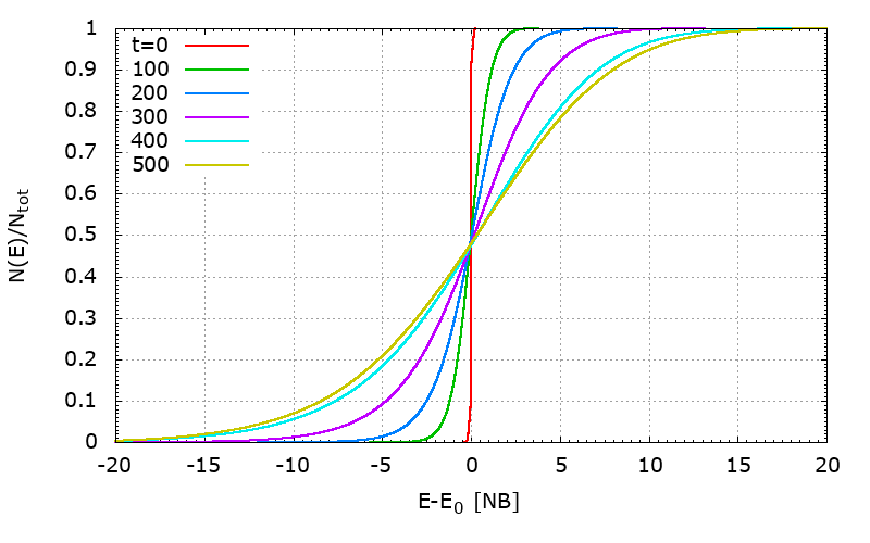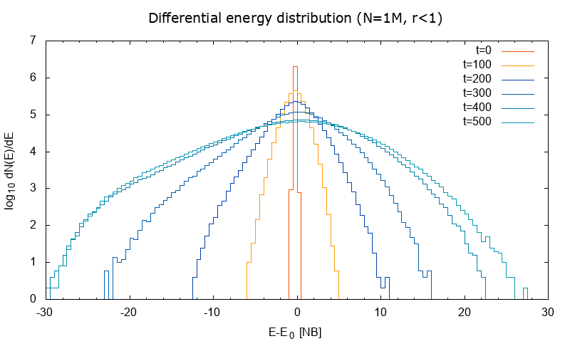
Figure 3. Differential energy distribution (similar to BT, p. 385):

Angular momentum diffusion

Figure 4. This is how the angular momentum distribution spreads with time. This one is for 1M run, \(L_\textrm{circ} = 5.0323\):

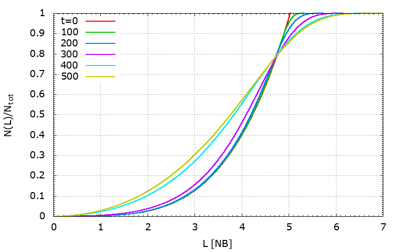Figure 5. Differential angular momentum distribution:

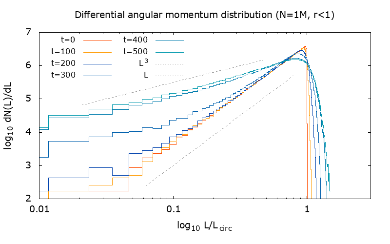Figure 6. Spreads of the energy \(\Delta E/E\) and angular momentum \(\Delta L/L\) vs time (UPD Oct 03: curves of run-06-xxx are added):

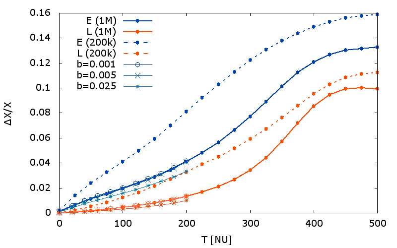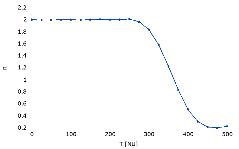
Figure 7. 'Effective’ index \(n\) of the model measured by fitting to the angular momentum distribution for \(0\leq L/L_\textrm{circ} \leq \frac34 \):

Even if the resonance relaxation time is factor of 100 shorter, there is a considerable margin for instability to evolve. However, we observe a steady change of the macroscopic parameters on the timescales \(t \sim 100\).

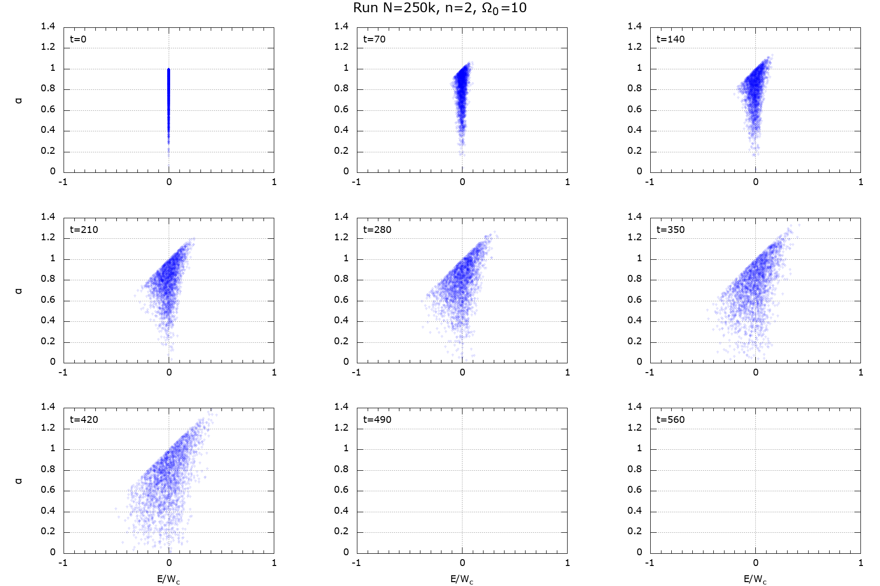
Figure 8. Spreading of the DF in E–L space:

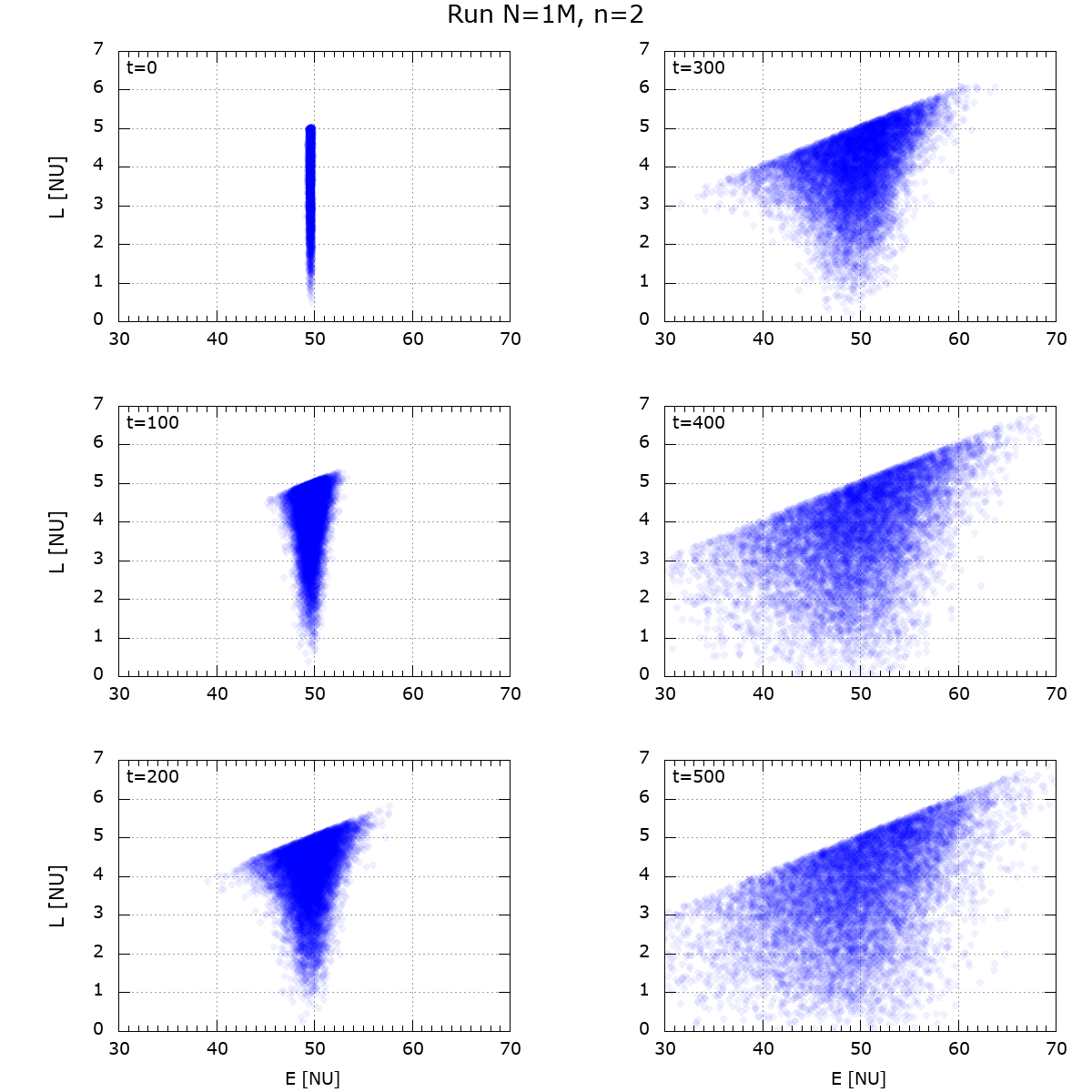Density, local anisotropy, relaxation time

Figure 8.

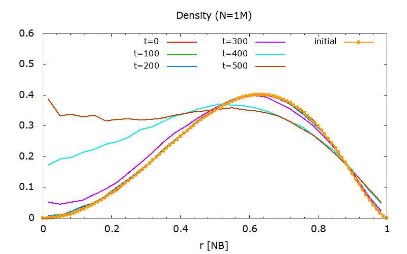Figure 9.

Figure 10.

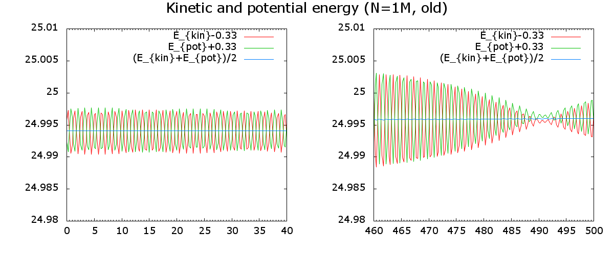
Figure 11.

A. Features:

1) Oscillations.

There are minor oscillations of kinetic and potential energies, which retain during simulations (Fig.11). They are present in the very beginning and do not disappear until the end of simulations.

2) Abnormal diffusion   t. The fast spread of the DF, and subsequent loss cone filling.

Figure 6 shows spread of the energy (standard deviation). It grows linearly with time, not like  sqrt(t) as it should be in standard diffusion.

3) Saturation of the instability.

We have a theoretical result for the growth rate of the loss cone instability in the limit of large \(\Omega_0\). I hope that the loss cone instability works even in the limit \(\Omega_0=0\). It is interesting if saturation takes place in models with smaller \(\Omega_0\) (less than 10).

4) Independence of the integrator.

Peter checked independence of the quadrupole amplitude curve of the integrator by comparing the default Leap-frog with Hermite and varying the timestep in Leap-frog.

B. Available runs and recent changes

I.

The first several runs were based on the old IPDs (initial particle distributions). These include a number of orbits in the library NL=1000, small errors resulting in a small fraction of particles near the circular orbit that does strictly obey \(E=E_0\) condition, lack of c.m. and total momentum correction to zero.

@ kepler, /home/Tit2/berczik/Evgeny-harm/, LEAP-FROG

a) (N = 200k):

old init… run-01 t_end = 10, dt_disk = 0.015625 = 1/64, dt = 0.000244140625 = 1/4096, eps = 5e-3

new init… run-02 t_end = 80, dt_disk = 0.250 = 1/4, dt = 0.000244140625 = 1/4096, eps = 5e-3 run-03 t_end = 80, dt_disk = 0.250 = 1/4, dt = 1/2048, eps = 5e-3 run-04 t_end = 80, dt_disk = 0.250 = 1/4, dt = 1/1024, eps = 5e-3

run-04 t_end = 80 - 500, dt_disk = 0.250 = 1/4, dt = 1/1024, eps = 5e-3

new dt/2
new2 dt*2

b) (N = 1M):

run-05 t_end = 500, dt_disk = 0.250 = 1/4, dt = 0.000244140625 = 1/1024, eps = 5e-3

new dt/2
new2 dt*2

@ laohu, NAOC, /ifs/data/peter/Evgeny-harm/laohu/run-laohu-01, HERMITE

N = 200k

II.

I updated IPD, using NL=10000, more accurate treatment of particles near the circular orbit so that now all particles obey \(E=E_0\), and Peter now makes the c.m. and total momentum correction. We have three 1M runs with T_max=500 and different eps.

run-06-0.001
run-06-0.005
run-06-0.025

III.

I updated IPD, using iterative correction of the density and potential for arbitrary \(\Omega_0\). This allows building fully self-gravitating systems.

Omega_0=0.00000, Nalp=10001

N=250000: E_kin=0.33353, E_pot=-0.66677, virial=-0.50023
N=500000: E_kin=0.33358, E_pot=-0.66679, virial=-0.50027
N=1000000: E_kin=0.33346, E_pot=-0.66673, virial=-0.50015
N=2000000: E_kin=0.33345, E_pot=-0.66672, virial=-0.50013

Omega_0=1.00000, Nalp=10001

Omega_0=3.16228, Nalp=10001

Omega_0=10.00000, Nalp=10001

N=250000: E_kin=25.33801, E_pot=24.32107, virial=1.04181
N=500000: E_kin=25.31377, E_pot=24.34516, virial=1.03979
N=1000000: E_kin=25.31895, E_pot=24.34001, virial=1.04022
N=2000000: E_kin=25.32714, E_pot=24.33188, virial=1.04090

I have generated 16 models, see /home/Tit5/epolyach/VW/Harmonic/harm_models.tar.gz

C. Plan:

1. Introduction // Loss cone and radial orbit instability - general criterium

1. Model description // model + growth rate for n=2

1. Theoretical explanation of fast diffusion // what to expect from Winberg 1998

1. N-body schemes // Leap-frog, Hermite integrators; softening; dt

1. Runs and results // describe how diffusion scales with N for different Omega_0; N = 250k, 500k, 1M, 2M; Omega_0= 0, 1, sqrt(10), 10

1. Discussion and conclusions

250k runs

Figure 12. Quadrupole amplitudes v.s. \(\Omega_0\)

Figure 13, 14. Smearing of the IPD due to centre of mass correction:

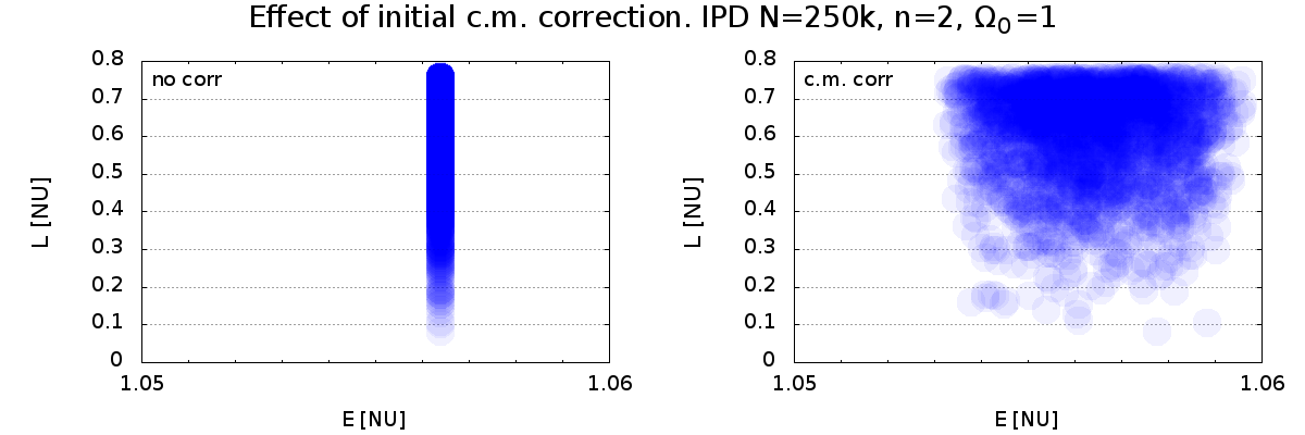Figure 15: \(\Omega_0=0\)

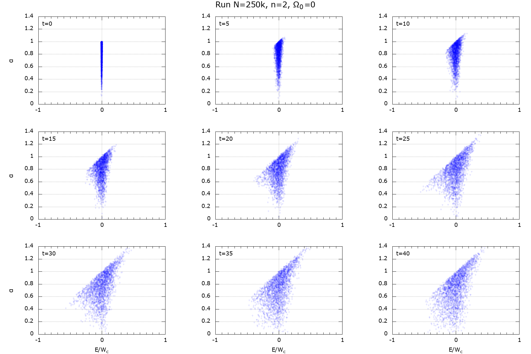Figure 16: \(\Omega_0=1\)

Figure 17: \(\Omega_0=3.16\)

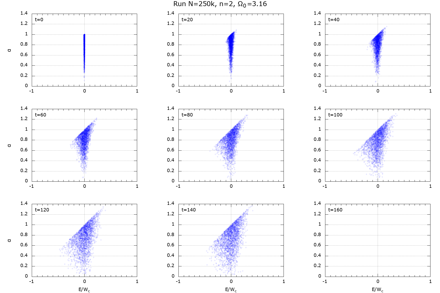Figure 18: \(\Omega_0=10\)

Energy diffusion

Here I calculated standard deviation as function of time for all 4 runs. Time is in units of \(T_0\) when the quadrupole amplitude for given \(\Omega_0\) attains maximum (Fig. 12; \(T_0=\) 25, 50, 100, 345, respectively). \(W_c\) is a virial of Clausius,

\[ W_c = |\sum_i m_i \mathbf{x}_i \cdot \mathbf{a}_i |\ , \]

equal to 0.669, 1.159, 5.651, 50.62, respectively.

Figure 19:

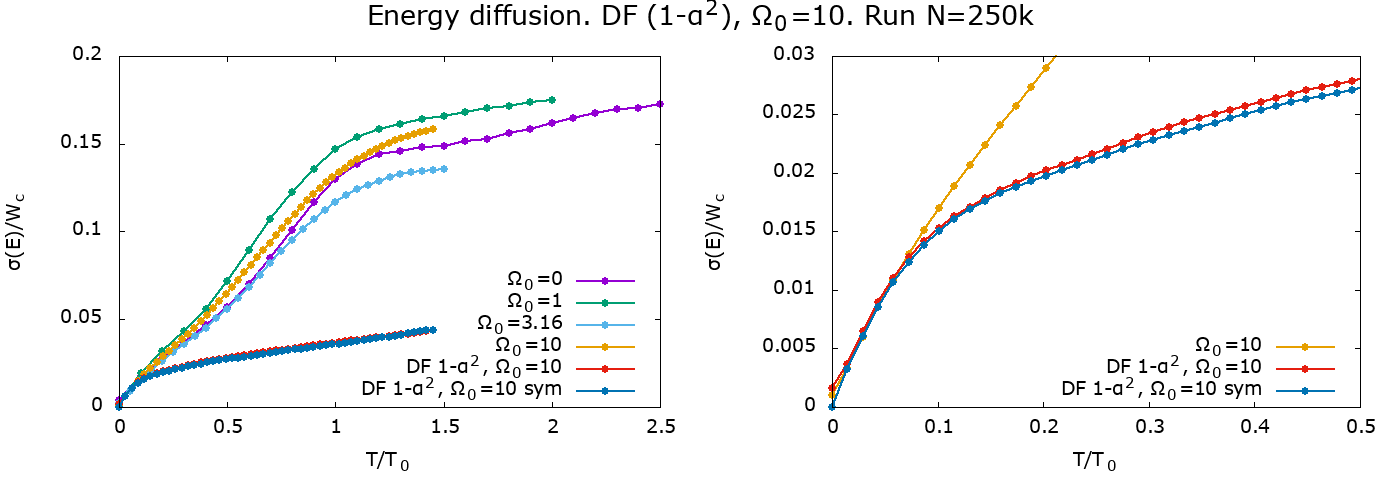Decreasing DF

We see that diffusion is abnormal even in the fully selfgravitating case. The congecture is that this is due to instability. We decided to simulate evolution of a stable model with DF \(f(\alpha) = 1-\alpha^2\).

Figure 20: \(\Omega_0=10\)

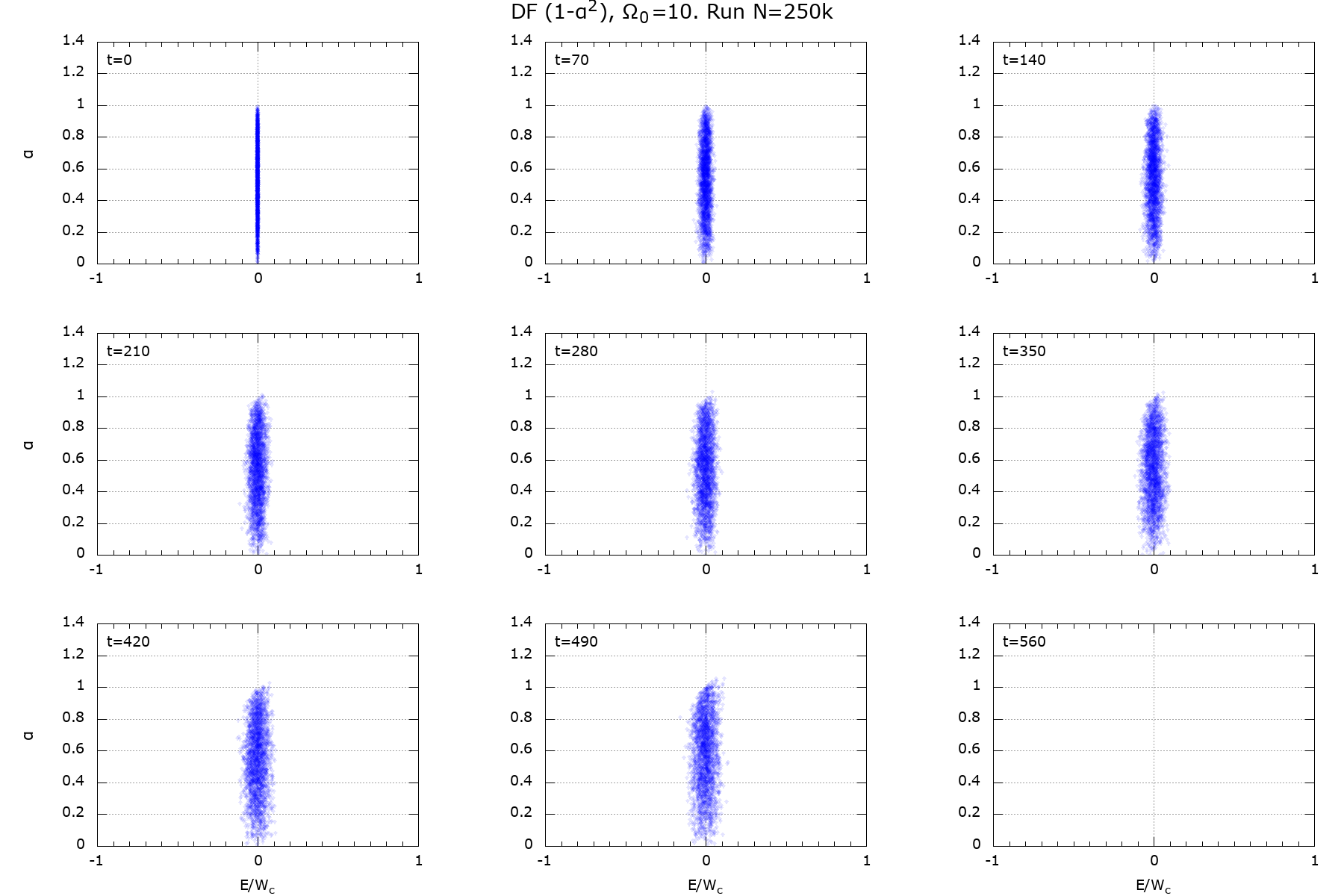Figure 21: Comparison of the energy diffusion for \(\Omega_0=10\), N=250k, with fits.

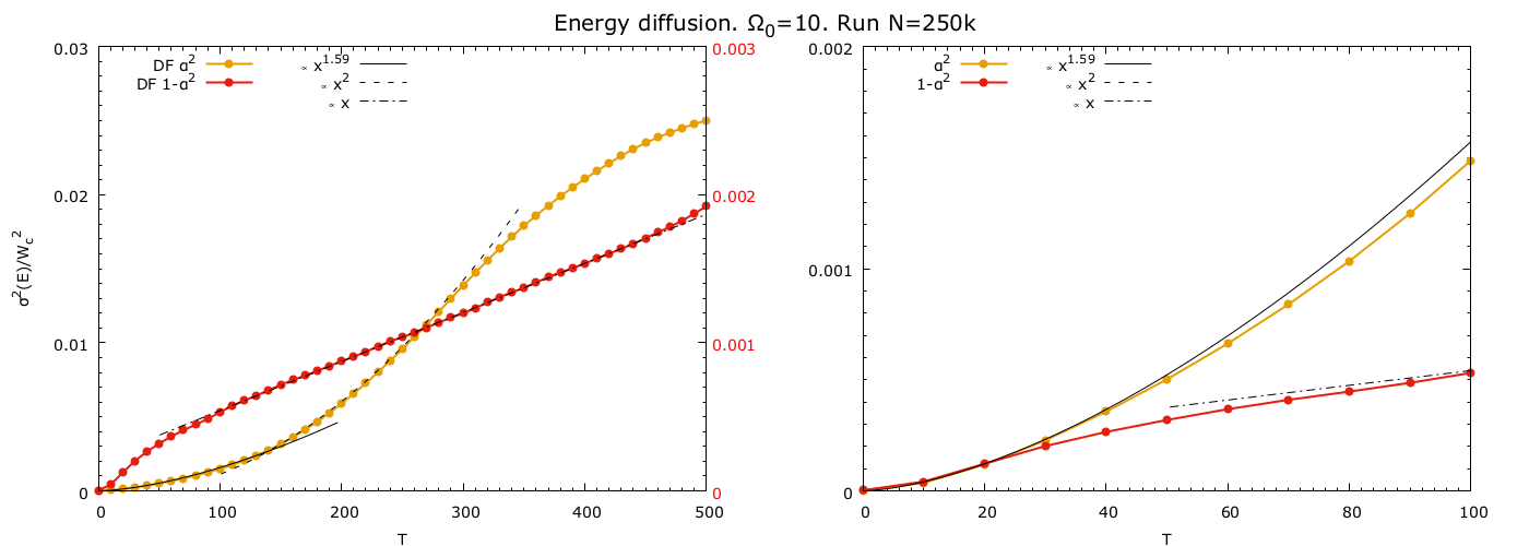Near-Keplerian case

Theoretical input

The power-exp model is

\[ \begin{equation} f(\alpha) = \frac{N}{\alpha_T^2} x^n \exp(-x) ,\quad x \equiv \frac{\alpha^2}{\alpha_T^2} \ . \label{eq:DF_pe} \end{equation} \]

It is assumed that this spherical stellar cluster is embedded to the dominating Kepler potential, so the total potential is

\[ \begin{equation} \Phi_0(r) = -G \frac{M_c}{r} + \Phi_G(r)\ . \label{eq:Pot_nk} \end{equation} \]

The mass of the cluster is

\[ \begin{equation} M_G = \int F d \Gamma = 2(2\pi)^3 \frac{dE}{\Omega_1(E)} \int\limits_0^{L_{\rm circ}} L dL \, F(E,L) \end{equation} \]

where \(F(E,L) = A\delta(E-E_0) f(\alpha)\), \(\int\limits_0^1 d\alpha \,\alpha f(\alpha)\).

\[ \begin{equation} A = \frac{\Omega_1 M_G}{16 \pi^3 L^2_{\rm circ} }\ . \end{equation} \]

\(R(E_0) = GM_c/|E_0|\)

\(\Omega_1(E_0) = (2|E_0|)^{3/2}/(GM_c)\)

\(\epsilon \equiv M_G/M_c\)

\(\overline{\omega} \equiv \omega / (\epsilon \Omega_1)\).

As a first step, we decided to model the simplest model with the maximum growth rate we :

Theoretical prediction of the growth rate:

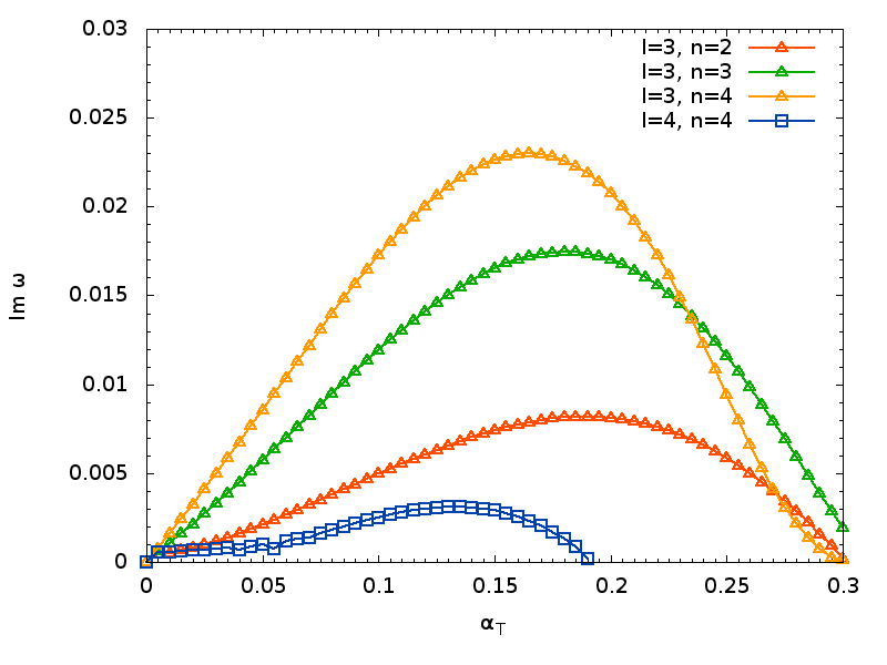As a first step, we decided to model the simplest Polyanomial DF: Theoretical prediction of the growth rate: