edita  >>> /home/epolyach/Data/WORK/Warp/TOOLS/Torque; /home/epolyach/Dropbox/WORK/WARP; /mnt/epolyach/Kepler/WARP/REZA

Warp paper with A. Just and R. Moetazedian

Comoving and inertial frames. Correction function

Often, it is convenient to calculate physical quantities in the comoving frame fixed at the density centre (d.c.) or the centre of mass (c.m). This comoving frame is not inertial in general. Below we shall denote quantities in the comoving frame with primes ’, while the corresponding quantities in the inertial frame will be without primes. E.g. position, velocity and acceleration of particle \(i\) are

\[ \begin{equation} \vec{x}_i = \vec{X} + \vec{x’}_i\ ,\quad \vec{v}_i = \vec{V} + \vec{v’}_i\ ,\quad \vec{a}_i = \vec{A} + \vec{a’}_i\ . \end{equation} \]

Figure 1: The shift of the comoving frame \(\vec{X}\).

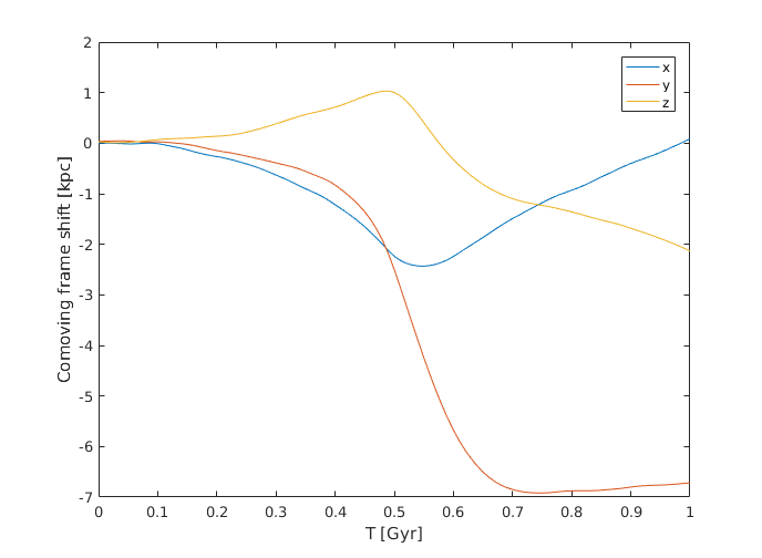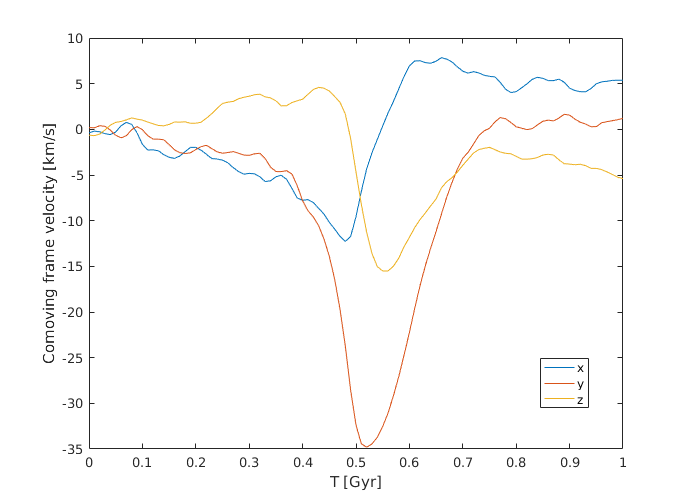
Figure 2: Associated velocity \(\vec{V}\).

Any numerical code assumes that the frame is inertial. So independently of the amount subtracted from particle positions and velocities, accelerations are the same. Thus ber-torque in the comoving frame calculates:

\[ \begin{equation} \vec{L’} = \sum\limits_{i} m_i \vec{x’}_i \times \vec{v’}_i \end{equation} \]

for angular momentum of particles and

\[ \begin{equation} \vec{M’} = \sum\limits_{i} m_i \vec{x’}_i \times \vec{a}_i = \sum\limits_{i} m_i \vec{x}_i \times \vec{a}_i - \vec{X} \times \sum\limits_{i} m_i \vec{a}_i = \vec{M} - \vec{X} \times \sum\limits_{i} m_i \vec{a}_i \end{equation} \]

for the torque (\(\vec{a}_i\) as in the inertial frame).

Now let's assume that conservation of momentum and angular momentum is perfect, and from equation \(\vec{M} = d\vec{L}/ d t\) in the inertial frame one should have:

\[ \begin{equation} \Delta \vec{L} \equiv \left. \sum\limits_{i} m_i \vec{x}_i \times \vec{v}_i \right|_t - \left. \sum\limits_{i} m_i \vec{x}_i \times \vec{v}_i \right|_0 = \int\limits_0^t dt \sum\limits_{i} m_i \vec{x}_i \times \vec{a}_i \ . \end{equation} \]

and

\[ \begin{equation} \vec{L} = \sum\limits_{i} m_i \vec{x’}_i \times \vec{v’}_i + M_d \vec{X} \times \vec{V} + \sum\limits_{i} m_i \vec{x’}_i \times V + \vec{X} \times \sum\limits_{i} m_i \vec{v’}_i \ , \end{equation} \]

where \(M_d\) is the disc mass. If \(\vec{X}\) and \(\vec{V}\) are c.m. position and velocity, then the last two terms vanish, i.e.

\[ \begin{equation} \vec{L’} = \vec{L} - M_d \vec{X} \times \vec{V}\ . \end{equation} \]

Let's introduce \(\vec{A}\):

\[ \begin{equation} \sum\limits_{i} m_i \vec{a}_i = M_d \vec{A}\ . \end{equation} \]

For the angular momentum change in the comoving frame, one obtains assuming \(\vec{X}(0) \approx 0\):

\[ \begin{equation} \Delta \vec{L’} = \vec{L}(t) - \vec{L}(0) - M_d \vec{X}(t) \times \vec{V}(t) = \int\limits_0^t d\tau \vec{M’}(\tau) - M_d \left(\vec{X}(t) \times \vec{V}(t) -\int\limits_0^t d\tau \vec{X}(\tau) \times \vec{A}(\tau) \right) \ . \end{equation} \]

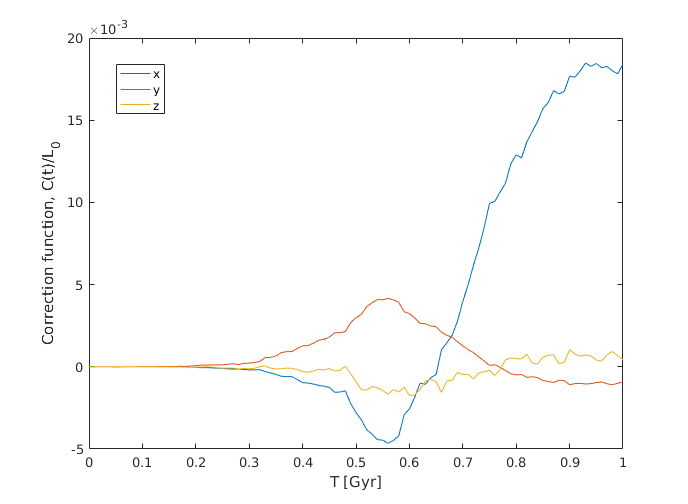
Here we have the correction term that takes into account non-inertial frame associated with the c.m. of the disc:

\[ \begin{equation} \vec{C}(t) \equiv -M_d \left(\vec{X}(t) \times \vec{V}(t) -\int\limits_0^t d\tau \vec{X}(\tau) \times \vec{A}(\tau) \right) \ . \end{equation} \]

Figure 3: Correction function (9) normalized to the initial angular momentum of the disc, \(L_0 = |\vec{L}(0)|\).

Whole disc: angular momentum change and time integrated torque

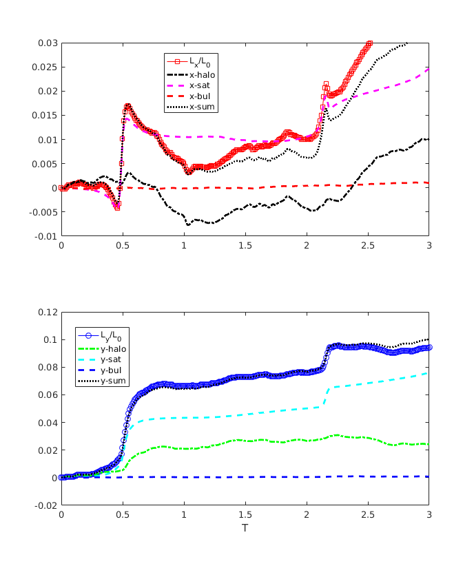
Calculations with ber-torque in the comoving frame associated with the c.m., however, show that change of the angular momentum in the l.h.s. is close to the r.h.s. without any correction term, i.e. as if the angular momentum and the torque are calculated in the inertial frame:

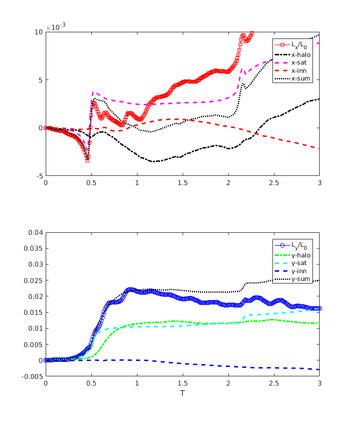
Figure 4: Change of the disc angular momentum (X and Y components) and the integrated torque from the halo, satellite and bulge. Proximity in X component is perfect up to 1 Gyr, for Y component – up to 2.2 Gyr. Bulge particles have low impact to the angular momentum balance, as expected.

Outer disc (R>15 kpc): angular momentum change and time integrated torque

For the outer disc, we calculate contributions of the halo, satellite, and the inner disc, R<12 kpc. Proximity in X component is perfect up to 0.5 Gyr, for Y component – up to 1 Gyr. There are waves on both \(L_x\) and \(L_y\) curves (radial waves seen in Reza's figures?).

Figure 5: The same as in Figure 4, for the outer disc. Again, correction term (9) spoils the proximity, as for the whole disc.

Torque from the spherical harmonics of the potential

The gravitational potential

\[ \begin{equation} \Phi(r, \theta, \varphi) = \sum\limits_{l,m} \Phi_{l,m}(r) Y_l^m(\theta, \varphi)\ . \end{equation} \]

The torque from the potential to a particle at \(\vec{r}\):

\[ \begin{equation} \vec{\tau}/m = - \vec{r} \times \nabla \Phi \ . \label{eq:torque} \end{equation} \]

In spherical coordinates:

\[ \begin{equation} \nabla = \hat{e}_r \frac{\partial}{\partial r} + \frac{\hat{e}_\theta}{r} \frac{\partial}{\partial \theta} + \frac{\hat{e}_\varphi}{r \sin\theta} \frac{\partial}{\partial \varphi}\ , \end{equation} \]

where unit vectors \(\hat{e}\) obey the relations:

\[ \begin{equation} \hat{e}_r \times \hat{e}_\theta = \hat{e}_\varphi\ , \quad \hat{e}_r \times \hat{e}_\varphi = -\hat{e}_\theta\ . \end{equation} \]

Substituting to (11), one has:

\[ \begin{equation} \vec{\tau}/m = - \hat{e}_\varphi \frac{\partial \Phi}{\partial \theta} + \frac{\hat{e}_\theta}{\sin\theta} \frac{\partial \Phi}{\partial \varphi} \ . \label{eq:torque_1} \end{equation} \]

Dipole

Now consider a torque from the dipole, \(l=1\), to a circular orbit. Let's write explicitly the spherical functions and derivatives:

\[ \begin{equation} Y_1^0 = \sqrt{\frac{3}{4\pi}} \cos\theta\ ,\quad \frac{\partial}{\partial \theta} = - \sqrt{\frac{3}{4\pi}} \sin\theta\ ,\quad \frac{\partial}{\partial \varphi} =0\ . \end{equation} \]

\[ \begin{equation} Y_1^1 = -\sqrt{\frac{3}{8\pi}} \sin\theta\,{\rm e}^{{\rm i}\varphi}\ ,\quad \frac{\partial}{\partial \theta} = -\sqrt{\frac{3}{8\pi}} \cos\theta\,{\rm e}^{{\rm i}\varphi}\ ,\quad \frac{\partial}{\partial \varphi} ={\rm i} Y_1^1\ . \end{equation} \]

\[ \begin{equation} Y_1^{-1} = \sqrt{\frac{3}{8\pi}} \sin\theta\,{\rm e}^{-{\rm i}\varphi}\ ,\quad \frac{\partial}{\partial \theta} = \sqrt{\frac{3}{8\pi}} \cos\theta\,{\rm e}^{-{\rm i}\varphi}\ ,\quad \frac{\partial}{\partial \varphi} =-{\rm i} Y_1^{-1}\ . \end{equation} \]

When averaging over \(\varphi\), one should remember that \(\hat{e}_\varphi = \hat{e}_y \cos\varphi - \hat{e}_x \sin\varphi\). Consider the disc plane, \(\theta=\pi/2\), and averaging along ring orbits (i.e., over \(\varphi\)).

• Let's analyse the first term in the r.h.s. of (14):

  • term with \(\Phi_1^0\) vanishes because of \(\hat{e}_\varphi\) dependence of \(\varphi\)

  • terms with \(\Phi_1^{\pm 1}\) vanishes because of \(\cos\theta\)

• The second term in the r.h.s. of (14) vanishes because of \({\rm e}^{\pm{\rm i}\varphi}\)

We conclude that the dipole component does not contribute to the orbit's tilting.

Quadrupole

Now consider a torque from the quadrupole, \(l=2\), to a circular orbit. Let's write explicitly the spherical functions and derivatives (\(c\) denotes \(\cos\theta\), \(s\) denotes \(\sin\theta\)):

\[ \begin{equation} Y_2^0 = \sqrt{\frac{5}{4\pi}} (3c^2-1)/2\ ,\quad \frac{\partial}{\partial \theta} = \sqrt{\frac{5}{4\pi}} 3c(-s)\ ,\quad \frac{\partial}{\partial \varphi} =0\ . \end{equation} \]

\[ \begin{equation} Y_2^1 = \sqrt{\frac{5}{24\pi}} (-3cs) {\rm e}^{{\rm i}\varphi}\ ,\quad \frac{\partial}{\partial \theta} = \sqrt{\frac{5}{24\pi}} {\rm e}^{{\rm i}\varphi} (-3c^2+3s^2)\ ,\quad \frac{\partial}{\partial \varphi} = {\rm i} Y_2^1\ . \end{equation} \]

\[ \begin{equation} Y_2^2 = \sqrt{\frac{5}{96\pi}} (3s^2) {\rm e}^{2{\rm i}\varphi}\ ,\quad \frac{\partial}{\partial \theta} = \sqrt{\frac{5}{96\pi}} {\rm e}^{2{\rm i}\varphi} (6cs)\ ,\quad \frac{\partial}{\partial \varphi} = 2{\rm i} Y_2^2\ . \end{equation} \]

• Let's analyse the first term in the r.h.s. of (14) for the quadrupole:

  • term with \(\Phi_2^0\) vanishes because of \(\cos\theta \)

  • terms with \(\Phi_2^{\pm 1}\) survive

  • terms with \(\Phi_2^{\pm 2}\) vanish because of \(\cos\theta\)

• the second term in the r.h.s. of (14) vanishes because of \(m{\rm e}^{\pm{\rm i}m\varphi}\)

We conclude that only terms with \(\Phi_2^{\pm 1}\) contribute to the torque:

\[ \begin{equation} \langle \vec{\tau}/m \rangle = - \left\langle \hat{e}_\varphi \frac{\partial \Phi}{\partial \theta} \right\rangle = -2 \sqrt{ \frac{15}{8\pi} } \left\langle \hat{e}_\varphi \Re \Phi_2^1{\rm e}^{{\rm i}\varphi} \right\rangle \ . \end{equation} \]

Let's introduce the complex phase \(\psi\): \(\Phi_2^{\pm 1} = |\Phi_2^{\pm 1}| {\rm e}^{{\rm i}\psi} \),

\[ \begin{equation} \langle \vec{\tau}/m \rangle = - \sqrt{ \frac{15}{8\pi} } |\Phi_2^1|\, ( \hat{e}_y \cos\psi + \hat{e}_x \sin\psi ) \ . \end{equation} \]

Odd spherical harmonics

\(P_l^1(\cos\theta)\) for odd \(l\) are equal to \(\sin\theta\) multiplied to a polynomial of \(\cos\theta\). Thus their \(\theta\)-derivatives vanish at \(\theta = \pi/2\) and no odd harmonics contribute to the tilt.

Even spherical harmonics

The \(\theta\)-derivatives of \(P_l^1\) are not zero. For \(l = 2k\), \(k=1,2…5\) at \(\theta=\pi/2\), they equal to 3, \(-15/2\), \(105/8\), \(-315/16\), \(3465/128\).

Comparison of the torque from the spherical harmonics with ber-torque calculations

Figure 6: 'q-h’ and 'q-s’ show contributions of the tilting torque (quadrupole term only) calculated w.r.t. the frame oriented so that z-axis coincides with the direction of the angular momentum vector of the inner disc, R<12 kpc. 'ber-h’, 'ber-s’, and 'total’ curves are the same as 'x(y)-halo’, 'x(y)-sat’, \(L_{x(y)}/L_0\) in Figure 4. 'ber-hs’ is a sum of 'ber-h’ and 'ber-s’. For halo torque, the proximity is amazing.

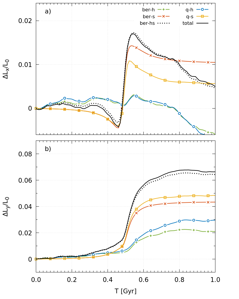Figure 7: Same as in Fig. 6, but for the sum of the even harmonics 2, 4 … 10 (instead of the quadrupole term). Comparison to Figure 6 shows that the quadrupole terms dominates in the tilting.